
A sense of uncertainty
In this second part of my informal three part mini-series on probabilistic machine learning, we will be looking at Bayesian Neural Networks, i.e. the result of probability theory taking an interest in deep learning. Be sure to also have a look at the first part, especially if you are unfamiliar with the basics of probability theory. As usual, you can have a look at the code I used to generate the figures for this article and also play around with it ![]() .
.
Some background
Let’s start with the topics that won’t be covered but for which I’ll supply some resources so you can brush up your knowledge if needed (just click on the small black arrow below). If you are like me and long resource lists give you anxiety because you feel obliged to read, watch and understand all of it before you can even start reading the article (which often results in an infinite regression into the depth of the Internet), don’t. Just pick whatever looks interesting or especially unclear or simply start reading the article and come back to the resources if something doesn’t make sense.
Show resources
Linear algebra & calculus: Okay, I know, you see this everywhere and for me at least, it always feels discomforting. What is it supposed to mean anyway? Do I need to know all of linear algebra and calculus to understand anything? And what does “know” mean? That I can solve matrix multiplications, determinants, Eigenvectors and 10th degree derivatives by hand in a few seconds? That I can proof the fundamental equations that underlie those fields? I don’t think so.
Usually, and this is also true here, it just means that you have an intuitive understanding of what is happening when multiplying a vector and a matrix or what a 2nd order derivative represents. Luckily, this kind of understanding can be obtained conveniently and even enjoyably by watching the following three video series (by one of my YouTube idols 3Blue1Brown who we will probably encounter again and again throughout this section and even throughout this blog):
- Probability theory: As you might have expected from the introduction, where there is Bayes, probability theory can’t be far. Again, an intuitive understanding will suffice to grasp what’s going on. Consider having a look at my article on the topic, which is intended specifically as a primer to probabilistic machine learning.
- Seeing theory
- Probability explained
- Bayes theorem and its proof (optional)
- Visual Information Theory (optional)
- Neural Networks: This is the second ingredient next to probability theory you need to construct a Bayesian Neural Network. 3Blue1Brown one more time.
- Machine Learning: Not strictly needed, but so cool that I need to share it. A visual introduction to machine learning: Part 1 and 2
What is this and why bother?
The first question coming to mind if confronted with the concept of a Bayesian Neural Network is, why even bother? My standard Neural Networks are working just fine, thank you! The answer is, that the world itself is inherently uncertain and a run-of-the-mill Neural Net has no idea what it’s talking about when it classifies your cat as a Ferrari with $99.9\%$ certainty.
When confronted with a difficult problem like “What did you eat on Monday two weeks ago?” you will probably preface whatever answer comes to mind with a “I’m not quite sure but I think…” or “It could have been…”. A standard Neural Net can’t do this. It’s more likely to conclude “She often eats spaghetti, so that’s what it was!”
A note for the critical among you: You might object that even a standard Neural Network returns a score for each class it’s predicting and you might be tempted to treat those numbers as probabilities of being correct, but there are at least two problems:
- Theoretical: Simply squishing an arbitrary collection of numbers through a Softmax function doesn’t magically produce real probabilities.
- Practical: It has been observed time-and-again now, that modern deep Neural Networks are overconfident (a notion we will come back to soon) such that the “confidence” expressed by the “probabilities” of the output layer don’t match the networks empirical frequency of being correct. In other words: A prediction of $0.7$ or $70\%$ for the class
catdoes not translate into $70$ out of $100$ cat images being classified correctly.
The real world is ambiguous and uncertain in all sorts of ways due to extremely complex interactions of a large number of factors (think, e.g., weather forecasting) and because we only ever observe it through some kind of interface: a camera, a microphone, our eyes. Those interfaces, usually called “sensors” in robotics, have their own problems like struggling with low light or transmitting corrupted information. An agent, be it a biological or artificial, must takes those uncertainties into account when operating within such an environment.
Uncertainty flavors
Usually, uncertainty is put into two broad categories which makes it easier to think about and model. The first, often called model uncertainty1, is inherent to the model (or agent) and describes its ignorance towards its own stupidity. A standard neural net is maximally ignorant in that it chooses one, most likely way of explaining everything—which translates into one specific set of parameters or weights—and then runs with those.
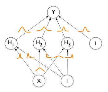
This is equivalent to an old person having figured out the answers to all the important questions and being impossible to convince otherwise. A Bayesian Neural Network, just as a biological Bayesian (the person), works differently. It considers all possible ways of looking at the problem2 and weighs them by the amount of evidence it has observed for each of those ways. It then integrates them into one coherent explanation. We will see what that looks like in practice a bit later. You can think about this as having a probability distribution for each weight (the little squiggly lines in yellow below) which determines the likely and less likely values each weight can take on. Usually, we have one multi-dimensional probability distribution for the entire network (where the number of dimensions equals the number of weights), also capturing (some of) the covariances between the weights.
The second type of uncertainty is commonly referred to as data uncertainty3 and it’s exactly what it sounds like: is the information provided by the data clearly discernible or not? You might think about a fogy night in the forest where you’re trying to convince yourself, that this moving shape is just a branch of a tree swaying in the wind. You can look at it hard and from multiple angles, possibly reducing your uncertainty about the thing (model uncertainty) but you can’t change the fact that it’s night, foggy and your eyes simply aren’t cut for this kind of task (data uncertainty). This also sheds light onto the fact that model uncertainty can be reduced (with more data) but data uncertainty cannot (as it’s inherent to the data).
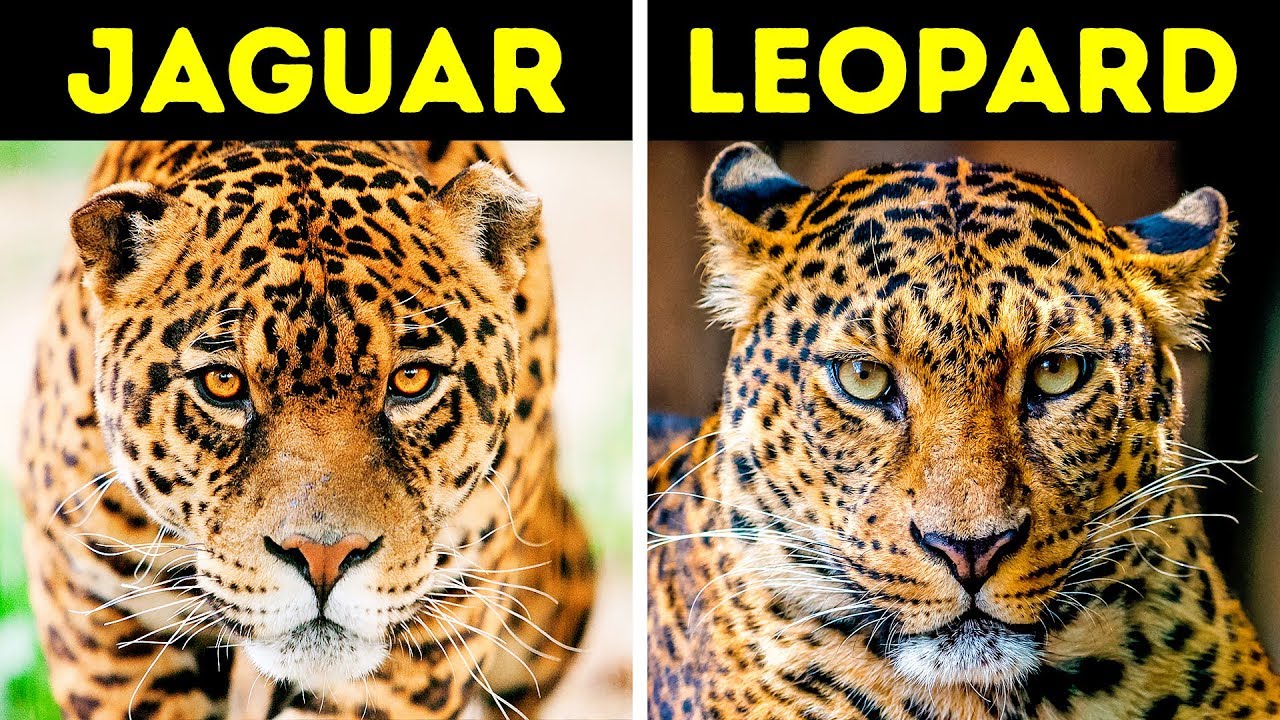
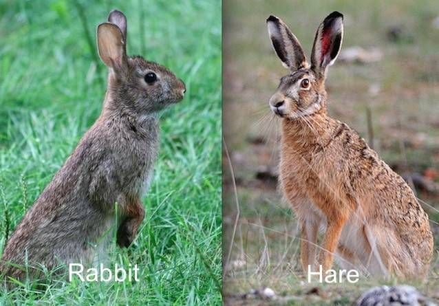
Below are some examples of data with low data uncertainty—the images are of good quality and the animals are clearly visible—but with a great potential for model uncertainty—though different, the animals look very similar, so we would need many examples to learn to differentiate between them.

Finally, both uncertainty flavors can be combined into an overall uncertainty about your decision: the predictive uncertainty. This is usually what one refers to when speaking about the topic of uncertainty and it is often simpler to obtain than the former two.
Modeling uncertainty
Now that we are certain about our need of uncertainty, we need to express it somehow. The only reason a human being doesn’t need a blueprint to do so is, that it has been indirectly hammered in by evolution and experience. In the sciences, this is done through the language of probability theory.
Before we can go any further, we need to sharpen up our vocabulary used to refer to specific things. Let’s first introduce our main protagonist: The neural network. It’s getting a bit more technical now, so feel free to review some of the necessary background knowledge if you’re struggling to follow.
Notation
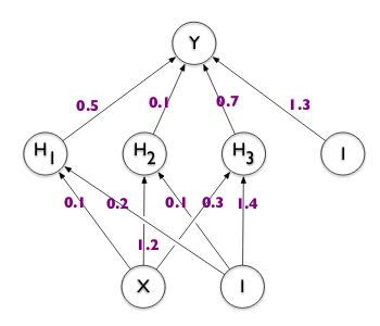
A neural network is a non-linear mapping from input $\boldsymbol{x}$ to (predicted) output (or target) $\boldsymbol{\hat{y}}=f_W(\boldsymbol{x})$, parameterized by model parameters (or weights) $W$, where we assume the true target $\boldsymbol{y}$ was generated from our deterministic function $f$ plus noise $\epsilon$ such that $\boldsymbol{y}=f_W(\boldsymbol{x})+\epsilon$. The entirety of inputs and outputs is our data \(\mathcal{D}=\{(\boldsymbol{x}_i,\boldsymbol{y}_i)\}_{i=1}^N=X,Y\), i.e we have $N$ pairs of input and output where all the inputs are summarized in $X$ and all the outputs are summarized in $Y$. Bold symbols denote vectors while UPPERCASE symbols are matrices.
Excursus: Images
In our case, the inputs are images and the outputs are vectors of scalars, one for each possible class (or label) the network can predict (e.g. cat and dog), so our network provides a mapping from a bunch of real numbers (the RGB values of the pixels of the image) to a number of classes. This means we are dealing with a classification rather than a regression problem.
If this all makes perfect sense to you, skip ahead to the next section, otherwise, let’s quickly explore how a computer can “see” images to then tell us what’s there to be seen. As computers can only deal with bits, everything we throw at them needs to be in this format. If we are working with numbers, that’s easy to do, but images?
The first thing we need to understand is, that an image is made up of pixels. And by understand I don’t mean to know the fact that this is so, but to grasp the implications of it. Each pixel has a name (or ID) and a color. The name is its position, usually given by a $x$, $y$ coordinate in a grid with rows and columns, but can also be a single number, if an additional order, e.g. from top left to bottom right is given. The color is usually made up of a mixture of red, green and blue (RGB), one set of primary colors from which we can mix every other color. So if we are given a $32\times 32$ pixel image, what we actually work with are $5$ numbers per pixel, the row and column coordinates as well as the red, green and blue color values, times the number of pixels which turns out to be $32\times32\times5=5120$ numbers.
If you hover over the first image below, the position and RGB color values of the currently selected pixel will appear. Due to the low resolution ($128\times128$), the pixels are already visible. By selecting a portion of the image (you can click and drag a rectangle), they will become even more salient. On the right, I’ve split the image further into it’s color channels (red, green, blue). By overlaying them, the original colors appear4, but if you rotate the image (by clicking and dragging), you will notice, that in fact there are only different shades of the primary colors. You can also zoom in here (by using your mouse wheel) to expose the individual pixels again.
Finally, the prediction made by the network is also just another number. We simply give each class a unique ID, e.g. cat becomes $0$ and dog becomes $1$. That way, everything is numeric again, and the computer is happy. Below are some additional ways of looking at the image introduced above. Just have a look around and continue once you are satisfied (or get bored).
Becoming Bayesian
So far, everything has been deterministic, which includes the weights $W$ of the neural network. But how do we actually know that those are the best possible weights? Actually, we don’t. We hope that they are reasonable by minimizing the loss during training. As you know, this is achieved by following the negative gradient (i.e. going in the direction of steepest decent) of the loss w.r.t. to the weights, using the backpropagation (i.e. the chain rule from calculus) algorithm to compute this gradient. Gradient descent optimization puts this aptly and succinctly.
Below is a loss landscape obtained by exploring a small area around the minimum found through gradient descent5. If you are interested in this kind of visualizations, have a look at this paper and the accompanying code.
What you might not know, if you haven’t been exposed to probabilistic machine learning, is, that gradient descent optimization is equivalent to maximum likelihood estimation in statistical inference. Imagine you want to find a friend on a large ship. You don’t know where she is but you think some locations, like the restaurant or the sun deck, are more likely than others, like the rear or the engine room. To quantify your uncertainty, you can use the tools of probability theory and model your world view as a probability distribution. If locations you deem likely are in the middle of the ship and less likely once are at the front and rear, you could, for example, use a normal distribution (aka Gaussian distribution or simply Gaussian in the machine learning community) centered at the middle of the ship to reflect this. What we just did is called modeling of a parameter, the location of your friend, and the probability you assigned to each possible location is called prior probability (or just prior), because it is your belief about the world before having observed any evidence (or information, or data) was observed.
Now imagine someone told you she was seen at the rear of the ship. This is a new piece of information which you should incorporate into your belief in order to maximize your likelihood of finding your friend efficiently. As the explanation already gave away, the probability to obtain this new information given your current belief about the parameter(s) you are trying to estimate is correct, is called likelihood.
Both of these terms, prior and likelihood, also appear in the probabilistic interpretation of neural network training. The information we base our beliefs about the likelihood of specific parameter configurations on is the data $\mathcal{D}$, while those parameters are the weights $W$. The difference to the deterministic setting is now, that we don’t work with a single set of most likely weights $W^\star$, but with a distribution over all possible weight configurations $p(\mathcal{D}\vert W)$, i.e. the likelihood function. We can still find the most likely set of weights though, by looking for the maximum of the likelihood as $W^\star=\arg\max_W p(\mathcal{D}\vert W)$, i.e. maximum likelihood estimation.
Why is this identical to gradient descent optimization now? Because, as it turns out, the typical loss functions used in neural network training, which are the cross entropy loss for classification and mean-squared error loss for regression problems, both have a probabilistic interpretation as the negative log likelihood, i.e. the negative logarithm of the likelihood! And because the logarithm preserves critical points and we minimize the negative likelihood in gradient descent optimization, this is the same as maximizing the actual likelihood in maximum likelihood estimation.
Mean-squared error:
\[E(W)=\frac{1}{2}(\boldsymbol{y}-\boldsymbol{\hat{y}})^T(\boldsymbol{y}-\boldsymbol{\hat{y}})=-\ln\mathcal{N}\left(\boldsymbol{y}\vert\boldsymbol{\hat{y}},\beta^{-1}I\right)\]Cross entropy:
\[E(W)=-\sum_{c=1}^K\boldsymbol{y}_c\ln\boldsymbol{\hat{y}}_c=-\ln\mathrm{Cat}(\boldsymbol{\hat{y}})\]As you might have glimpsed from these equations, the mean-squared error can be interpreted as the negative logarithm of an isotropic multivariate normal distribution of the true labels centered around the predictions with precision $\beta$ while the cross entropy has an interpretation as the negative logarithm of a categorical distribution of the predictions.
To obtain the likelihood given the loss, we can simply solve the equation $E(W)=-\ln p(\mathcal{D}\vert W)$ for this quantity to obtain $p(\mathcal{D}\vert W)=\exp(-E(W))$. Below, on the left, you see a visualization of taking the exponential of the negative loss while on the right, a fitted two-dimensional normal distribution is shown. Interestingly, they are extremely similar, suggesting to use such distributions when trying to model the likelihood functions of neural networks, a fact we will come back to in the final article of this series when talking about Laplace approximation.
For now, simply have a look at (and play with) the figures and try to understand the relationship between loss and likelihood. For example, regions of low loss indicate parameters (network weights) of high likelihood and flat regions of the loss translate to high uncertainty about the correct parameter values, as many different configurations are equally likely to have generated the data.
We have discussed the loss-likelihood relation so let’s turn to the prior. As the prior encompasses all assumptions about the parameters we want to estimate, almost everything that is known as regularizers in standard machine learning lingo can be cast into this framework. Those are basic things like the choice and design of our model, i.e. using a neural network and giving it a specific number of layers and other architectural decision but also, more explicitly, regularization of possible values we allow the weights to take on, the most common being weight decay, aka $L_2$-regularization, where larger values are penalized. Especially this last example, again, has a specific probabilistic interpretation, becoming a Gaussian prior in the probabilistic context.
Introducing a prior into the mix elevates our maximum likelihood estimate to a maximum a posteriori estimate, owing to Bayes’ theorem, telling us that the posterior distribution is proportional to the likelihood times the prior, i.e. $p(W\vert\mathcal{D})\propto p(\mathcal{D}\vert W)\cdot p(W)$. So while gradient descent optimization performs maximum likelihood estimation absent any form of regularization, it seamlessly elevates to maximum a posteriori estimation once regularization is introduced where the optimal weights are found by maximizing the posterior instead of the likelihood such that $W^\star=\arg\max_W p(W\vert\mathcal{D})$.
Bayesian Inference
Bot the maximum a posteriori and the maximum likelihood estimate are so called point estimates. This makes sense, because even though we have modeled the weights probabilistically, we don’t make full use of the fact by then reducing the likelihood or posterior distributions to a single, most likely value $W^\star$ through maximization.
We can now simply plug those weights into our network and perform inference: Making predictions on new, unobserved data. This final step however can also be performed in a proper probabilistic way, through marginalization: removing the influence of a random variable by summing (if discrete) or integrating (if continuous) over all of its possible values. Suppose we are given a new datum, e.g. an unobserved image of an animal $\boldsymbol{x}^\star$, for which we would like to predict the class $\boldsymbol{y}^\star$. Using deterministic inference, we would simply use our neural network with trained weights:6
\[\boldsymbol{y}^\star=f_{W^\star}(\boldsymbol{x}^\star)\approx p(\boldsymbol{y}^\star\vert\boldsymbol{x}^\star,W^\star)\]In Bayesian inference, we are not using the best weights, instead we are using all possible weights. This means we don’t need to keep them around any longer, having extracted all the information we could, so we end up with just $p(\boldsymbol{y}^\star\vert\boldsymbol{x}^\star)$. How can we obtain this? We can start by adding everything else we are given, apart from the new input, namely the rest of the data and our neural network, i.e. the weights. Now we have $p(\boldsymbol{y}^\star\vert\boldsymbol{x}^\star,W,\mathcal{D})$. But the predicted class of the new image doesn’t depend on the data we’ve received so far, so we can split the expression into $p(\boldsymbol{y}^\star\vert\boldsymbol{x}^\star,W)\cdot p(W\vert\mathcal{D})$. The first term is our neural network: Given an image and a set of weights, it can predict class probabilities. The second term is the posterior: Telling us how well our chosen model parameters (the weights) can explain the evidence we have seen (the data). If we want to get rid of the influence of the weights, which, after all, are just an arbitrary choice we’ve made to model the problem, we can integrate them out:
\[p(\boldsymbol{y}^\star\vert\boldsymbol{x}^\star)=\int p(\boldsymbol{y}^\star\vert\boldsymbol{x}^\star,W)p(W\vert\mathcal{D})\mathrm{d}W\]Both deterministic as well as Bayesian inference finally use the most likely class, i.e. the maximum of $\boldsymbol{y}^\star$, as the prediction.
Going further
So far we have looked at different kinds of uncertainty and why they are important, similarities and differences between deterministic and Bayesian neural networks, the relationship between the shape of the loss landscape and our uncertainty about the optimal parameters and how to make predictions the Bayesian way.
What’s left now to put all of this into practice is a way to precisely estimate the likelihood (or posterior) of our network and then, using this knowledge, to make reliable predictions with reasonable confidence. As this involves solving the—unfortunately intractable—integral above, we will also look at Monte Carlo integration as a feasible approximation. Those are the topics of the next and final article of this series. More specifically, we will explore Laplace approximation for deep neural networks, how it is used and finally some results from the work I did for my Master’s thesis including some code examples to bridge the gap between theory and application. See you there!
-
Or epistemic uncertainty. ↩
-
Within the limited pool of possibilities granted to it during its design, captured by the choice of possible probability distributions used for modeling the likelihood of the weights. ↩
-
Or aleatoric uncertainty. ↩
-
The colors are not identical to the original image on the left, because the blending of colors is done through transparency instead of actual mixture of the color channels. ↩
-
Keep in mind, that this is a low dimensional representation of the true loss surface, which has as many dimensions as the network has weights ↩
-
Not the $\approx$ because a neural network doesn’t provide actual class probabilities in general. ↩