
Truly understanding 1x1 convolutions
In this short post we will finally understand $1\times1$ convolutions. I say finally, because I’ve thought many times now that I had understood them only to find a use-case where their application again didn’t seem to make sense.
My insufficient understanding stemmed of course from insufficient engagement, for which I’m to blame, but also from deficiencies in the explanations I found. While trying to understand the PointNet architecture for deep learning on point clouds for example, I was again mystified by the concept of a “shared MLP” (multi-layer perceptron) “sliding” over the input and how it was implemented using convolutions. Because the explanatory content became too long for a simple interlude inside another article, I decided to devote a full post to the subject.
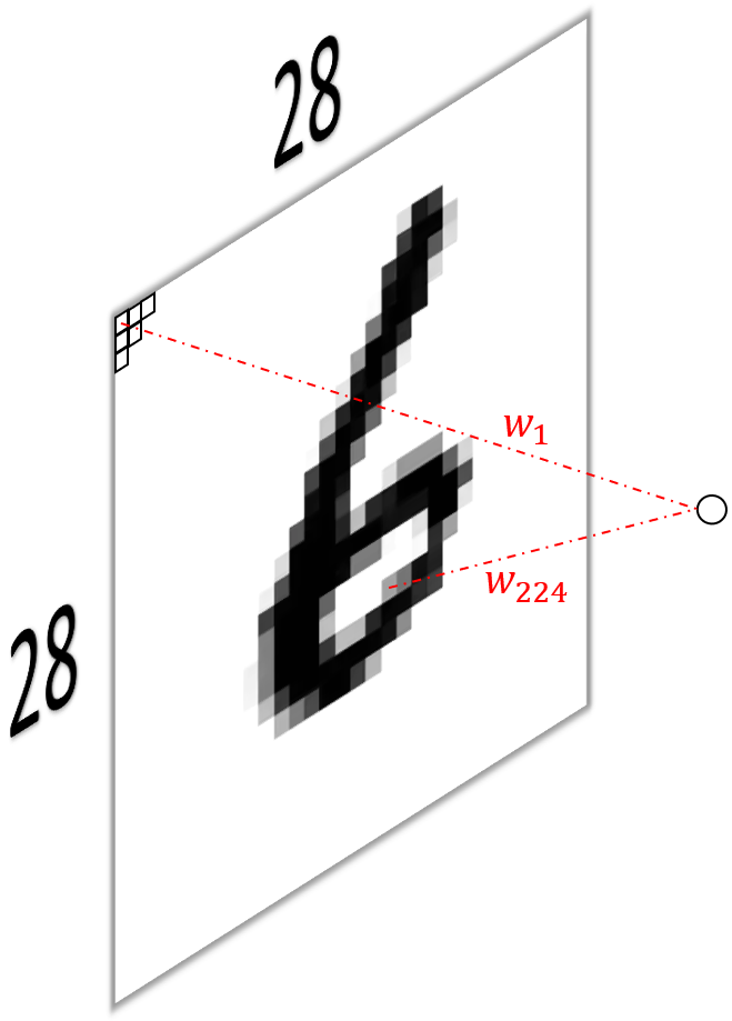
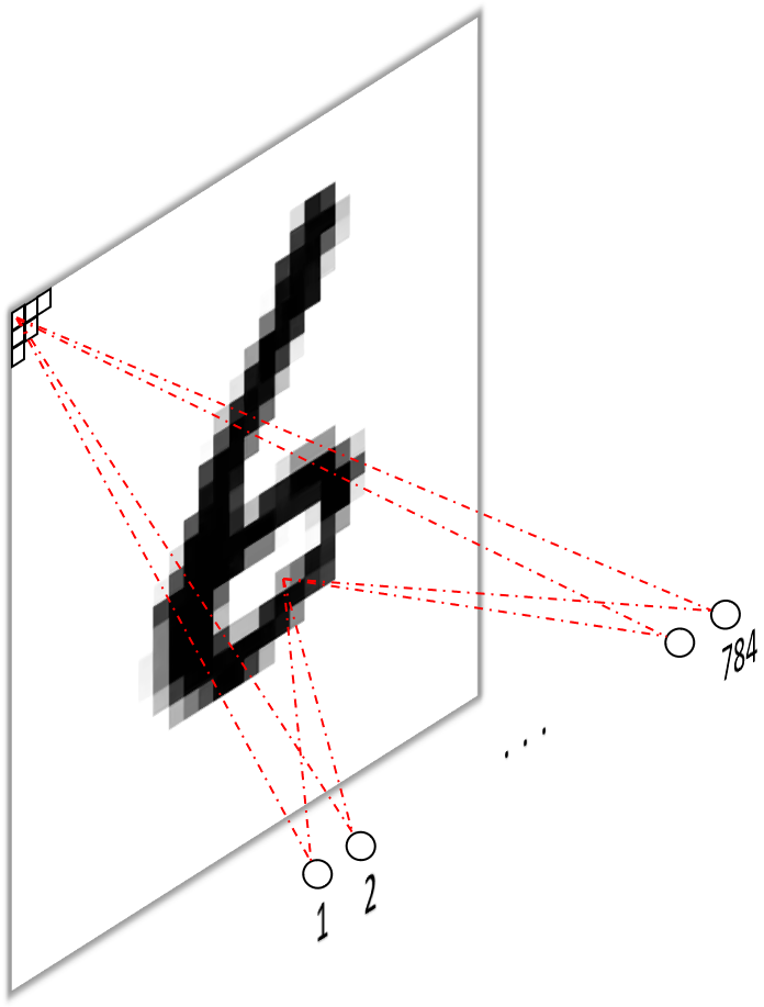
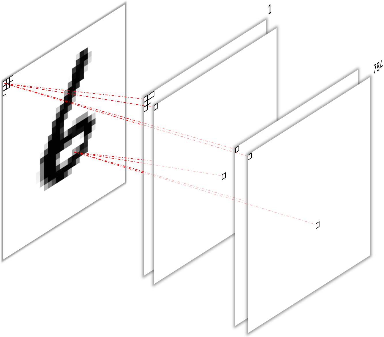
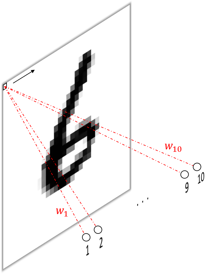
To get started, let’s quickly recap how a fully connected layer1 would operate on a monochrome (black and white) image. Below (figure 1) I’ve visualized how a single neuron (a) and an entire fully connected layer (b) operates on such a $28\times28=784$ pixel image. The mathematical operation performed by each unit in this layer is
\[y=\sum_{i=1}^{784}w_ix_i+b,\]where $b$ is an offset, usually called the bias (not shown in the figure). This means we obtain $784$ scalar outputs $y$ from the layer, one from each unit.
Now let’s see how we can mimmick these operations using convolutions. In what follows, I’m assuming some basic familiarity with (convolutional) neural networks on your part. If that’s not the case, have a look at the background section of one of my previous posts or this excellent explanation from the famous CS231n Stanford course to brush up your knowledge.
To learn from images, we present them, one by one or in batches of multiple images, to a stack of convolutional layers, each consisting of a stack of filters in turn. This exploits the structure of images, where neighboring pixels are assumed to be highly correlated, to reduce the number of parameters compared to a fully connected approach, where each pixel gets its own weight.
A standard convolutional layer is defined by the number of input channels, e.g. the red, green and blue color channels of an image for the input layer, the height and width of the kernels or weight matrices (we have one kernel per input channel) which are convolved with the input channels to give the convolutional neural network its name, and the number of output channels, or feature maps, or filters. A convolutional layer operating on an RGB image with $3\times3$ kernels and 128 filters would therefore be of dimension input channelxkernel heightxkernel widthxoutput channel i.e. $3\times3\times3\times128$. The first dimension is usually omitted, as it is deemed obvious (i.e. easily inferred from the number of channels from the input) and the output channel are sometimes stated in the first (“channels first”) or last (“channels last”) position. Below (figure 2) you see a simple convolution on a monochrome (black and white) input image (a) and the conceptually easy to imagine implementation using a “sliding fully connected” network (b).
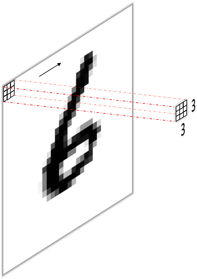
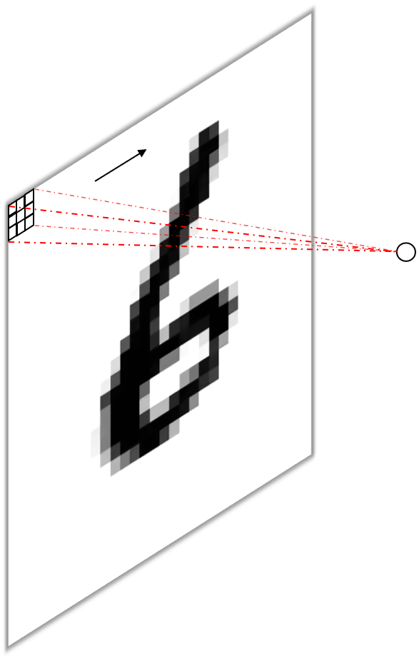
The idea of sliding a small network over the input, as shown in fig. 2 (b), initially introduced in the Network in Network paper, seems quite intuitive. If you were to actually implement this though, you would notice that it’s a non-trivial task, because both “sliding” and “only being partially connected” are not part of the standard repertoire of a fully connected layer. Instead, let’s try to express a fully connected layer as a convolution, which slides and partially connects natively. To do so, we have two options:
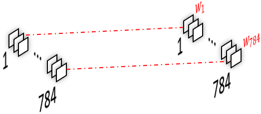
- Using one filter per input pixel with one large kernel ($28\times28$) per input channel (figure 3).
- Using one filter per input pixel with one small kernel ($1\times1$) per input channel and pixel (figure 5).
I think the first approach is relatively intuitive. The convolution operation performed by each filter is identical to that stated above for a single fully connected unit, i.e. multiplying a unique scalar weight with each input pixel and summing them up. Consequently, we obtain the same $784$ scalar outputs, one from each filter, perform the same number of operations (multiplications and additions) and have the same number of parameters ($784\times784=614656$ omitting biases).
If we reduce the width and height of our filter kernels to one, we obtain $1\times1$ convolutions. Let’s first look at a trivial example (figure 4) with a single filter and three kernels, operating on an RGB image (a) and again the conceptually simple extension to the fully connected approach (b).
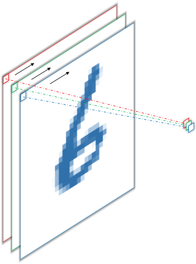
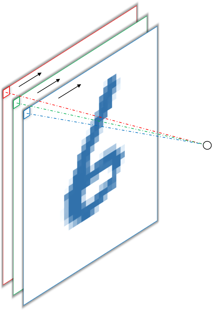
The important thing to note here is, that both approaches produce a single output per spatial dimension (i.e. width and height), because, per convention2, convolutions of input channels and kernels from the same filter are summed up, meaning each filter only produces one feature map. In the example above, the red, green and blue pixel values are multiplied by the red green and blue weights and then summed to give a scalar output. This is actually the more common way to employ $1\times1$ convolutions, namely as a way to reduce or increase depth, i.e. the number of output channels and not to mimic fully connected operations. For example, we can put this to use in the final layer of our network to produce one feature map per class by sliding $10$ filter with $1\times1$ kernels over the output feature maps of the previous layer. In the figure below (6), this would produce one feature map for each digit from one to ten, where each “pixel” in the feature map corresponds to the “oneishness” or “twoishness” of each input pixel3.
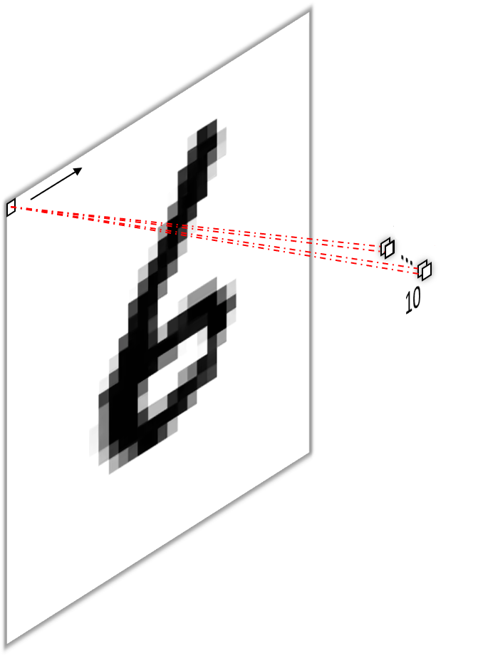
Armed with the knowledge from the previous paragraph, we can now understand the second approach of transforming a fully connected layer into a convolutional layer. To do so, we first transform the image into a vector4 by concatenating all of its pixels and then apply one filter per pixel with one kernel per pixel, as our image now has as many channels as it had pixels (i.e. it is of shape $1\times1\times784$). Have a look at figure 6 below to take it in visually.
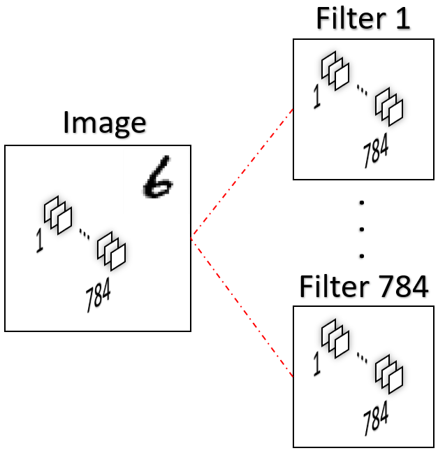
Because each filter produces a single scalar (as input dimensions are summed), we again end up with $784$ outputs. So it’s actually not as simple as exchanging the fully connected layer by a $1\times1$ convolution to gain the same functionality. Instead, we need to first reshape the image and then apply as many filter as there are pixel in the input.
That’s it! If there are other ways to understand $1\times1$ convolutions, better ways to visualize them or any mistakes, please let me know. I hope this really cleared things up for you as it did for me when writing and visualizing the subject.
-
Also often called dense layer. ↩
-
This part is often omitted! ↩
-
Interestingly, summing those feature maps over the spatial dimensions would again produce the same result as a fully connected layer, i.e. one scalar value per class, so we could view it as a third way of mimicking fully connected layers with convolutions. ↩
-
Another important information often omitted (or not considered?) in the explanations I found on the subject. ↩