
Learning from Point Clouds
It’s a great achievement to have found an algorithm that can solve problems on its own (more or less) by simply dropping a huge pile of data on it and telling it what we want to know. In the grand scheme of things this is known as machine learning though nowadays it mostly means deep learning.
Deep learning is named after its champion, the deep neural network, which enjoys a formidable renaissance since a couple of years. Mostly though, the deep learning revolution has been taking place in a very specific domain, namely that of images, which we could also refer to as ordered 2D RGB point clouds, as you might recall from the previous post.
From our perspective though, the world is arguably more three dimensional–or even four if you’re Einstein–than flat. Naturally, one might wonder why we haven’t heard more about advances in 3D deep learning. For once, the data acquisition is not as smooth yet compared to images. Almost everyone has access to a rather high quality camera by reaching into their pockets, but only in recent years have sensors to capture the third dimensions become somewhat affordable in the form of RGBD (D for depth) cameras in gaming consoles.
And then there is the computational overhead. Adding a dimension to our data increases computational demands exponentially, rendering most real world tasks infeasible. This is slowly beginning to change though, so it might be an excellent time to dive into this exciting field of research, which I intend to do in this article. We’ll be looking at various ways of learning from 3D data which have been proposed over the last couple of years, sorted by the way they represent the third dimension: Point clouds (1), Voxel grids (2), Meshes and Graphs (3) and multiple (2D) views (4). Unsurprisingly, we start with number one, the point cloud and tackle the others in later articles.
Can’t be that hard, right?
As discussed in the previous article, point clouds are great, as they are the most natural data representation, directly obtained from our sensors. They are inherently sparse and therefore space-saving, but they also come with some problems. The first is varying density, i.e. some regions feature significantly more points than others, and secondly lack of order. Both effects are visualized below. Contrary to images, the shape of the point clouds, and therefore the object it represents, is preserved no matter in which order its points are stored and presented. Were we to reverse the order of pixels in an image we would flip it horizontally (i.e. perform a $180°$ clockwise rotation), while shuffling the pixels would results in garbage (noise).
On the left, you see the point cloud of the Stanford Bunny1. Points are distributed uniformly over its entire surface. On the right you see the same bunny, but with two important differences:
- Points vary in density, leaving some areas empty while others are covered well. This resembles the kind of point clouds obtained from range scans in the wild more closely.
- The order of the points has been reversed. Imagine we color each point by the position in the $N\times3$ vector in which the point cloud is stored (this means we assume $N$ points with $3$ dimensions, i.e. $x, y, z$ coordinates each) and that point $1$ is closest and point $N$ is furthest away (which produces the depth image, where close points are bright and far points are dark). Reversing the order of the points in the vector but keeping the coloring scheme, we now get dark points in front and bright points at the rear, though the shape of the bunny is unaffected. In fact, any other permutation of the points in the vector would give the same shape (but different coloring), because a point in a point cloud is not defined by its position in the underlying data structure but by its coordinates in space. This is what’s meant by the term permutation invariance and it’s a concept our deep learning algorithm needs to learn in order to classify point clouds robustly.
A third problem pose rigid motions. Rigid motions are a subset of affine transformations, including translation and rotation. Rotation invariance on images is often improved by augmenting the training data with small random rotations, while translation invariance is an inherent feature of convolutions. Both are infeasible in three dimensions because we’re dealing with three rotation axes as opposed to one (requiring exponentially more data augmentation to cover the same range of motion) and we can’t convolve the point cloud because it’s unordered (see problem 2).
Due to these difficulties, most previous approaches pre-processed the point clouds either into voxel grids, meshes or collections of 2D images from multiple perspectives (views) to then use more traditional 2D and 3D convolutional neural networks on them. Let’s now have a look at how those problems have been tackled in research.
1. PointNet
In the pioneering architecture for learn directly on point clouds, PointNet, the authors only focused on the second and third problem, namely permutation and transformation invariance, tackling varying density in their second work, which we’ll come to right after. Instead of blindly following the story as told in the paper, let’s instead focus on the individual problems of learning from point clouds and the proposed solutions.
1.1 Solving transformation invariance
If we can’t learn something implicitly from data, we need to build it into our model explicitly. In PointNet, this is achieved through a small sub-network which learns to predict a $3\times3$ rotation matrix which is then applied to the point cloud. This allows the network to align each object in a way it sees fit. While the first transformation is applied to the input (in three dimensional input space), it is later repeated in $64$ dimensional feature space (giving rise to a $64\times64$ matrix). Because learning a useful transformation matrix in this high dimensional space is more challenging, the authors constrain it to be close to an orthogonal matrix by adding an $L_2$-like regularization term. These small sub-networks are trained end-to-end with the rest of the network, even though they solve a regression task (finding $9$ and $4096$ real numbers respectively) instead of the overarching classification (or segmentation) task.
Interestingly, this increased the accuracy by “only” $2\%$, but I’m guessing that the training data was already relatively homogeneous and that improvements could be bigger on less uniform or more corrupted real world data.
1.2 Solving computational complexity
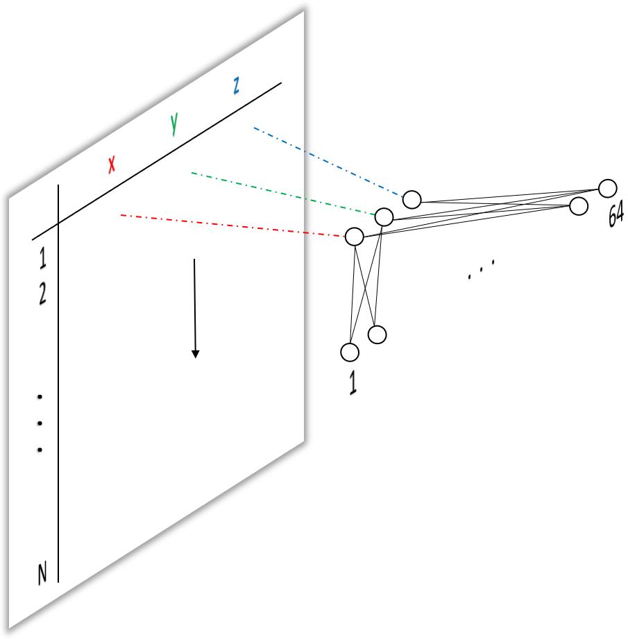
Now that our point cloud is oriented correctly, we need to classify it. If we were to naively implement a neural network to do so, we would need $N\times3$ input units (neurons), as we can’t use convolutions on unstructured data, because they inherently assume that neighboring points (or pixel) are correlated, while, as discussed above, the order of points in a point cloud is arbitrary. Apart from the immense computational complexity for large $N$ (large point clouds with many points), we would have to train one network per point cloud size or sub/super sample each input to have exactly the same number of points (this is commonly done when pre-processing images for classification, though not for semantic segmentation).
Another idea would be, to “slide” a network with $3$ inputs, one for each spatial dimensions, over each of the $N$ points. This is what’s meant in the paper where the authors introduce the concept of a shared MLP. MLP being multi-layer perceptron, i.e. a network with fully connected layers2 only. This means we share one network for all $N$ points in the point cloud. This is exactly what the input to a network classifying individual points instead of point clouds would look like.
Let’s have a closer look at sharing and sliding. If the notion of sliding weights over inputs, performing multiplications and additions sounds familiar to you, that’s because it’s the definition of a convolution! But wait, didn’t I just discredit convolutions for the use on point clouds? Well, bear with me for a second. As it turns out, we can replace a fully connected layer by a convolutional layer with $1\times1$ kernels. If this doesn’t make sense to you, and it didn’t for me in the beginning, I invite you to take a look at my previous post where I take a deep dive into the application of $1\times1$ convolutions.
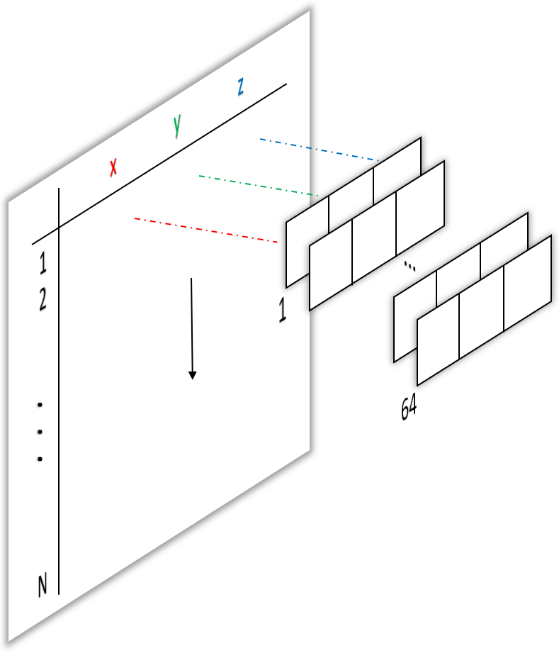
On the input layer, we can replace our fully connected layer from figure 1 with a $1\times3$ convolutions, i.e. 64 filter with one $1\times3$ kernel each, as shown below.
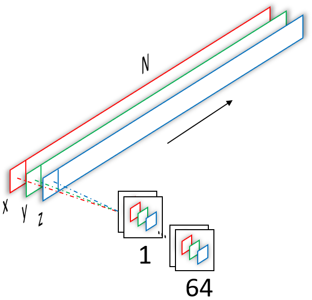
We could also use a second approach of employing $1\times1$ convolutions, which actually is used deeper in the network, but this would require us to reshape the point cloud from $N\times3\times1$ to $1\times N\times3$ beforehand (again, please have a look at the previous post if this doesn’t make any sense to you). To the contrary, once we have convolved our input with the $1\times3$ convolutions, the output is one scalar value per filter, i.e. of dimension $1\times1\times64$, exactly what we need to now use $1\times1$ convolutions on it (and get the same behavior as a fully connected layer)!
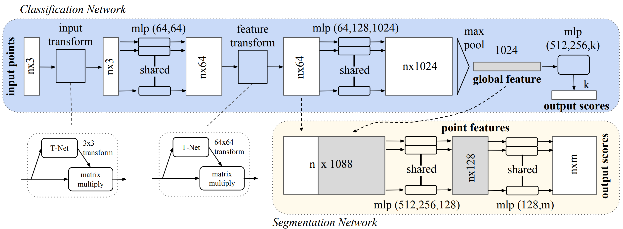
If we now have a look at the entire network architecture as presented in the paper (figure 4 below), the term mlp(64,64) begins to make sense. Instead of using an actual MLP with $3$ input units, $64$ hidden units and $64$ output units, we use a convolutional network with two layers of $64$ filters each, where each filter in the first layer has one kernel of size $1\times3$ (figure 2) and each filter in the second layer has $64$ kernels, each of size $1\times1$.
1.3 Solving permutation invariance
As discussed above, we want our network to predict the same class, no matter in which order the points are presented. Can you think of a function (aka a mathematical operation) that produces the same result, independent of the input order (i.e. that is commutative)? Turns out, there are many and its super simple. Here is one: $4+3+1=3+1+4$. Addition. Here is another: $2\times8=8\times2$. Multiplication. The authors opted for the $max$ operator, i.e. $max(5, 7, 10)=max(7,5,10)=10$.
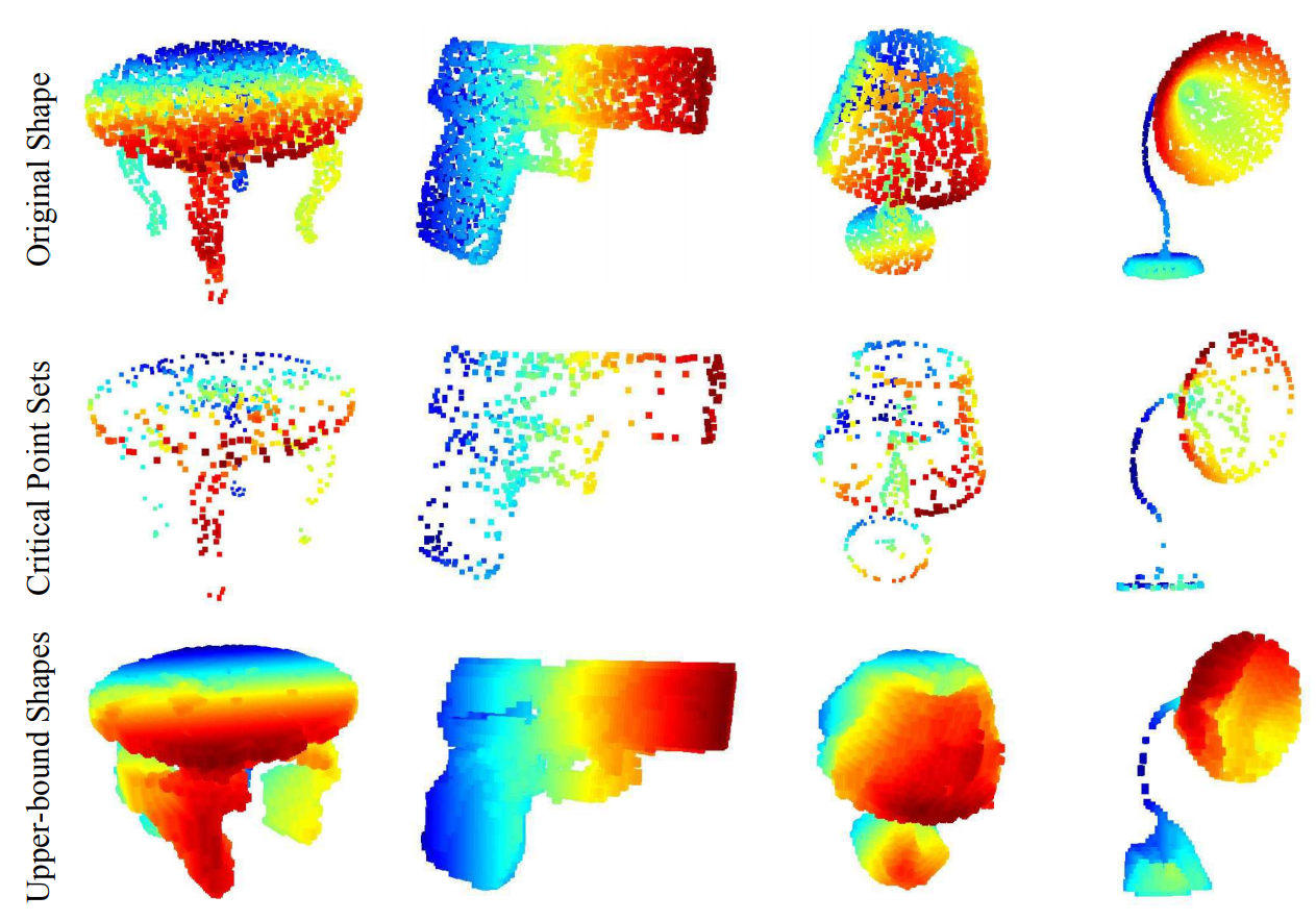
This has the added advantage that the network is pushed to reduce each object to its most important features, as is the case when using max-pooling in convolutional networks, which leads to increased robustness to outliers, missing points and additional points, because the result will be the same as long as the most descriptive points remain. Interestingly, those turned out to be the skeletons of the objects (figure 5).
In figure 4 you see the max operation applied towards the end of the network, transforming local features (per point) to global features (for all points, i.e. for the entire point cloud). The final layer is an actual MLP then, without parameter sharing, as we don’t “slide” the network over each point independently, but just use the $1024$ dimensional global feature space. We could also use other classifiers on those global point cloud features like Support Vector Machines, but being able to train the network end to end and then also use it for inference is of course much more elegant.
1.4 Solving semantic segmentation
As you might have noticed, the authors use a second network architecture to perform semantic segmentation. Here, we need to classify each point into one of $K$ classes instead of the entire point cloud.
The segmentation network reuses the both local and global features computed by the classification network and concatenates them, as the semantics of a point are defined both by its immediate neighborhood (i.e. the part of an object or the object of a scene it belongs to) but also the class of the entire object or scene. You won’t find a wing as part of a table just as you won’t find a stove in the living room.
Apart from the output, which provides class scores per point, the architecture of the segmentation network is very similar to the classification network, also making use of the shared MLP idea.
1.5 Experiments and results
With all problems solved3 let’s see what can be done with PointNet. The authors test classification performance on ModelNet40, a dataset featuring CAD models of common objects like chairs, tables, cars and planes. They are on par or better than all previous approaches none of which used point clouds directly but multiple object views or voxel representations instead and significantly reduces inference time compared to deeper and more complex architectures.
Part segmentation is performed on the ShapeNet dataset which is similar to ModelNet40, just much larger and with added part labels. Again, previous approaches perform worse when comparing the mIoU (mean intersection over union) average of all classes. Especially interesting is the graceful decline in performance when using more realistic incomplete point clouds which is handled much worse by previous methods.
Finally, scene segmentation performance is reported on the Stanford 3D semantic parsing data, which consists of multiple rooms with objects such as chairs and tables and other semantic entities like floors and walls. Due to the lack of competition, the authors compare to a baseline with hand-crafted features which they outperform by a large margin, achieving a per-point accuracy of more than $78\%$.
The remainder of the paper focuses on ablation studies, validating various design choices such as max-pooling to achieve order invariance, the input and feature transformation and depth and width of the networks.
2. PointNet++
With such great results and so many great solutions to difficult point cloud problems you thought we were done, right? Far from it though! The most glaring omission in PointNet was the problem of varying densities as explained in the beginning. This is a very real problem with point clouds obtained from real world 3D scans. Usually, such point clouds are generated from a single depth image or stitched together from multiple depth images, though usually still from only a small range of viewpoints, leaving occluded regions completely blank.
In the image domain, a similar problem to varying density exists under the name level of detail. Depending on the resolution of your camera or the distance of an object to it, many or few pixel can be devoted to said object resulting in ample or meager information to judge it by. So maybe one could take inspiration from solutions developed in this domain? This was tackled in the subsequent work of the PointNet team, aptly titled PointNet++.
2.1 Density or Resolution?
Have a look at the point cloud below. From the current perspective, it’s not particularly dense, leaving ample space between the points. Now, see what happens as you zoom out; The point cloud seems to become denser! It’s not really of course, rather, we changed the resolution of our inquiry.
This is a slight shift in perspective4 which allows us to tackle the problem of varying densities through changes on our end, i.e. in the way we design our algorithm, instead of manipulating the point cloud itself. Let’s see what a naive approach could look like.
Say we partition the point cloud into spheres of varying size, starting from many overlapping small spheres and ending with one large sphere which encompasses the entirety of points. Now, we could feed all points in each sphere into the network and let it learn to identify local and global regions of the input as the same object.
The problem with this approach is twofold. Firstly, by processing each region independently, we lose cross-region information and secondly, we drastically increase computational complexity. In the image domain this is handled more efficiently by stacking multiple convolutional layers where layers deeper into the network have a larger receptive field5.
However, there is nothing stopping us from employing the same idea for point clouds! As we’ve seen in the first section of this article on PointNet, we’re already using convolutions on point cloud features, so by simply stacking multiple PointNets operating on various partitions of the input point cloud, we can achieve a similar effect as in convolutional neural networks.
2.2 Partitioning
Let’s see how the partitioning, called sampling & grouping in the paper, of the input point cloud is done in detail. There are three important choices to be made when dividing a point cloud into spherical regions: How many spheres, where to place them and which diameter. One and three are related, as we want to cover all points, so a decreasing number of spheres needs to result in an increase of diameter of each. Partitioning a space in this way is reminiscent of voxelisation, with the important difference, that the size of spheres is variable and that we don’t try to describe all points inside by the sphere itself but instead only use it to select a subset of points.
Problem two, i.e. where to place the spheres, is solved by the farthest point sampling algorithm. FPS is a recursive strategy, always finding the farthest point from all currently chosen points, as to cover the entire space most efficiently.
The pipeline then looks as follows. First we find the centroids of our spheres recursively using FPS until all points are covered, which generates a receptive field in a data dependent manner. Then, we find all points belonging to each region using ball query, which is standard nearest neighbor search but only inside the current sphere. A convolution on pixels basically does the same thing, the only difference is, that the neighborhood is measured by Manhattan distance instead of Euclidean distance. This approach guarantees fixed region scale which makes local region features generalizable across space, as opposed to directly relying on the K nearest neighbor algorithm around each centroid, which would make dense regions much smaller. Finally, PointNet is applied to each region, where point coordinates are expressed relative to the regions center. This allows to learn relations between points, which was missing from the initial PointNet architecture.
Repeating this approach for multiple sphere diameters results in what is called multi-scale grouping in the paper. This is computationally expensive however, as we are still dealing with one application of PointNet per sphere and diameter. Another idea is the use of multi-resolution grouping. Here, we exploit the fact that we already have computed features on small sub-regions in the previous layer, so by combining those sub-regions into one larger region we only need to compute new large-scale features on it and concatenate all results to obtain local and global information. Both approaches are visualized below.
In its entirety, the approach as described above results in one so called set abstraction layer, of which we can concatenate several to obtain a hierarchical architecture.
2.3 Experiments and results
Similar to the experiments in PointNet, PointNet++ is evaluated on ModelNet40 for classification and ScanNet for segmentation, outperforming the previous state of the art.
An additional interesting result was obtained on MNIST, converted into 2D point clouds, where the authors showed that PointNet++ is capable of outperforming the small convolutional LeNet5 network (though not larger CNNs), proving the effectiveness of an hierarchical approach for point clouds.
The most interesting results in my eyes are obtained on corrupted and thinned data. During training, the authors used random dropout of input points as an augmentation technique to force the network to learn density invariant features, which the architecture should hypothetically be capable of. Indeed, in contrast to the original PointNet as well as a 3D CNN operating on voxels, PointNet++ is almost unaffected by modest decreases in point denstity.
Wrapping up
That’s all for now. Next we’ll take a look at learning from structured data (voxel grids), graph neural networks, which try to exploit dynamically generated local graph structures or global graph information in the form of meshes to learn from 3D data and multi-view as well as projection-based approaches learning from the 2D domain. However, this post will be updated whenever I come across an interesting new architecture which can extract meaning directly from point clouds. Thanks for reading and see you soon in the next article.
Code: ![]()
-
I figured as we move to the academic setting in this post, we might as well use the standard academic example instead of the Happy Buddha from the last post. ↩
-
Also often called dense layers. ↩
-
Take this with a grain of salt, as “solved” only means that we are now able to do at least something rather than nothing at all. ↩
-
Pun intended. ↩
-
Though (random) cropping of images during training, and even sometimes during inference is additionally performed frequently. ↩