
Context
Welcome to this little journey where we discover some fundamental concepts in the realm of (machine) learning, namely context and attention. The story is told in two acts: 1. Why and 2. How. We will cover the why and the legacy part of how in this article and then take a closer look at a modern approach in the next one.
Why? Conceiving context
It all begins with a little entity making up most of the (digital) world around you. It takes many names some calling it word, pixel or point, but we will simply call it element. Our little element is secretive, revealing almost nothing about itself in isolation. In that regard, it is like its sibling in the real world, the atom. Both are atomic1. It has emergent properties though: Throw a couple of thousand of them together and you get a story, an image, a 3D model. What has changed? The Context.
Context: The circumstances that form the setting for an event, statement, or idea, and in terms of which it can be fully understood.
Let’s look at a couple of examples. The simplest (an therefore the one we will see most frequently throughout the article) is the word. Try to guess the meaning of the word below, then hover over it with your mouse (or tap on it) to reveal the context:

Did you guess the meaning correctly? Or was it the financial institution or place to sit? The point is, of course, that you couldn’t have known without the context of the entire sentence, as many words are ambiguous. It doesn’t stop there though. Even the sentence is ambiguous if your goal is to determine the book title or author who wrote it. To do so, you might need a paragraph, a page or even an entire chapter of context. In machine learning lingo, such broad context is commonly called a long-range dependency. Here is another one. Pay attention to the meaning of the word it:

Seeing tired, we know it must refer to the animal, as roads are seldom so while it’s the opposite for wide2.
Below, there are two more examples of increasing dimensionality (use the little arrows to switch between them). While sentences can be interpreted as one-dimensional sequences of word-elements, an image is a two-dimensional grid of picture-elements (pixels) and a 3D model can be represented by a cloud of point-elements3 (or volumetric-elements: voxels). You will notice that you can’t discern what is represented by the closeup view of the individual elements but when zooming out (using the “Zoom out” buttons and your mousewheel or fingers) the interpretation becomes trivial.
Again, context doesn’t stop there. To correctly place a pixel as belonging to, say, an eye, you need the surrounding pixels making up the eye. To place the eye as coming from an adult or a child you make use of the information stored in the pixels around the eye. Such inference can potentially go on indefinitely, but it’s usually restricted by the size of the depicted scene or the resolution of the image. Okay, you might think, so is more information always better? No.
Finding the hidden information in the image above is trivial if the surrounding context is removed (to be precise, it’s not the absence of context, as all pixels are still there, but the contrast between signal and noise, percieved as difference between gray and colored pixels). Clearly, it’s not a simple as having no context at all or all of it but rather which portion of the provided information we pay attention to.
How? Context across dimensions and domains
Now that you are hopefully convinced that context is an important concept across domains, let’s start this section off by investigating how researchers have dealt with it prior to the advent of attention. First up are sequence data in the form of written and spoken language. Then we will look at images and 3D data formats in turn.
Context without attention
For a long time, the predominant method used to model natural language was the Recurrent Neural Network (RNN), first in a basic fully-connected flavor and later using Long-Short-Term Memory (LSTM) and Gated Recurrent Units (GRU). In this paradigm, context is accumulated over time, one element (word) after another, allowing the model to reference potentially indefinitely into the past. Potentially, because in reality it turns out that the memory is rather short and plagued by vanishing and exploding gradients, a problem addressed to some extend by the LSTM and GRU variants. The recurrent nature, while interesting, also requires sequential computation, resulting in slow training and inference. Additionally, the model can’t look into the future,4 requiring a complicated encoder-decoder design, first aggregating the entire context of the input to provide the decoder with the necessary global context,5 a point we will return to in the last section of this article.

The shortcomings of RNNs motivated the look into alternatives, one of which was found in a revered companion: the convolution. At first glance, this might seem like a strange choice, considering convolutions as almost synonymous with locality. However, there are at least two tricks to aggregate long-range dependencies using convolutions. The first one is to simply stack them. Maybe due to their prevalence in image processing, the range covered by a convolution is called its receptive field and through stacking, it can be grown.
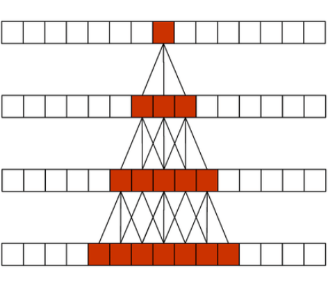
Now, for large inputs (a long text, a high resolution image, a dense point cloud), this simple way of increasing the receptive field size is inefficient, because we need to stack many layers which bloats the model. A more elegant way is to use strided convolutions, where the convolutional kernel is moved more than a single element, or dilated (atrous) convolutions, where the kernel weights are scattered across the input with perceptive holes (French: trous) in between. As we might miss important in between information with this paradigm we can again stack multiple such convolutions with varying strides or dilation factors to efficiently cover the entire input.
Moving to the image domain, there is no fundamentally new idea here as vision models still largely rely on convolutions with similar characteristics as introduces above, the only change being the added second dimension.

Adding a third dimension, things get more interesting again, as the computational complexity of convolutions becomes a major problem. While they can be used successfully, the input usually needs to be downsampled considerably prior to their application. Another approach is to use an element-wise feed-forward neural network6. This approach is extremely efficient, but doesn’t consider any context. To resolve this, context aggregation is performed by an additional process like Farthest Point Sampling, k Nearest Neighbor search or Ball Queries. One exception is the Graph Neural Network. As the name implies, it works on graphs as input (either dynamically computed or static ones as found in triangle meshes) and can leverage graph connectivity for context information. I’ve written an entire mini-series on learning from various 3D data representations which I invite you to check out if the above seems inscrutable.
Taming context with attention
Cliffhanger. See you in the next post.
References
| [1] | Understanding LSTM Networks |
| [2] | UNetGAN |
| [3] | WaveNet: A generative model for raw audio |
| [4] | Review: Dilated Residual Networks |
-
Not really of course, words can be divided into letters, atoms into particles, but let’s ignore that. ↩
-
This, and many more of these (deliberately) ambiguous sentences can be found in the Winograd schema challenge. ↩
-
Also known as a point cloud. Take a look at the previous articles on learning from 3D data for other representations. ↩
-
Except for bi-directional RNNs which read the sequence from left and right. ↩
-
An example being machine translation: The input sequence (a sentence in English) is first encoded from the first to the last element (word) and then decoded sequentially to produce the translation (the sentence in French). ↩
-
Sometimes referred to as shared MLP (Multi-Layer Perceptron), which in the end boils down to a 1x1 convolution as discussed here. ↩