
Learning from Graphs
Welcome to this third and still not final episode of the series learning from 3D data. We’ve already looked at point clouds, and voxel grids so now it’s time for graphs. I’ve already motivated learning on 3D data as opposed to 2D data like images here, so let’s skip this and directly move on to a quick recap on point clouds and voxels to see why we might want and need yet another representation.
Previously on 3D deep learning
Point clouds are great, because they are the raw output of 3D scanning hardware so we don’t need any hand-crafted pre-processing. Apart from being computationally efficient they are also efficient to store due to natural sparsity where unoccupied space remains empty and we simply store a three-tuple of xyz coordinates for each point. Extracting information from this format, i.e. learning, is however difficult in part due to this sparseness but also due to unorderedness and varying density.
Voxel grids try to alleviate some of these problems by putting points into boxes, i.e. voxels, and stacking them into an ordered structure, the voxel grid. Similar to images, each voxel now has pre-defined neighbors and density is equalized through binning, as multiple nearby points are lumped together into a single voxel. This allows to employ the workhorse of deep learning on 2D structured data, i.e. images, namely convolutions.
The holy graph
What do graphs bring to the table then? The best of both worlds would be an exaggeration, but there certainly is some of both. But what is a graph anyway?
Above, you see a part of a graph. The two basic building blocks are vertices1, the dots, and edges, the lines. As you can see, edges connect vertices, but not every vertex is connected to all others. This fact translates into structure, which is the first property graphs share with voxel grids, as each vertex has a pre-defined set of local neighbors. Compared to point clouds, such structure can help to separate semantically different parts of an object, like the left an right leg, even though they might be very close by in the observed Euclidean space.
If you look closely though, the structure imposed by a graph is also different from that of a voxel grid, as we are still left with varying density: some regions are covered more densely than others. This property, shared with point clouds, is a blessing and a curse. On the one hand it allows for efficient coverage of space, where highly detailed regions can be covered densely while uninformative regions are spanned by few vertices and edges or even none at all in the case of empty space. On the other, in conjunction with the missing order of neighbors, it prohibits the straight forward application of convolutions.
Ultimately, we want to learn local, stationary, and compositional features on graphs. You might not be aware of this, but all of these properties are fulfilled when learning on images using deep convolutional architectures. Localized information is only valid in an immediate vicinity, which is important, as we might need to learn different features to differentiate tails from ears. This property is taken care of automatically by using convolutional filters with fixed-size kernel matrices, extracting information from the immediate surrounding only. Stationary information remains discriminative regardless of the surrounding context. This property is often referred to as translation invariance, e.g. the ability to detect edges anywhere in an image using the same filter. Finally, compositional information allows to build up higher-level concepts from low level features, like geometric primitives from lines, eyes and ears from those primitives and faces from eyes, ears and noses.
If you zoom out on the visualization above, you see that the presented graph describes an object seen previously in this series: the happy Buddha from The Stanford 3D Scanning Repository. It also is a special kind of graph, where each vertex has exactly eight edges, and three edges form a triangle. This kind of structure is called a triangle mesh or simply just a mesh2, and it offers even more structure than a simple graph, which can be exploited intelligently as we will see later.
There are a couple of properties not necessarily visible in simple visualizations of graphs, two important ones being the directedness (or undirectedness), meaning an edge is a one-way street only traversable in one direction and weightedness, meaning each edge obtains a scalar weight value, signifying some property like length. A mesh for example is an undirected, unweighted graph. Apart from these invisible properties, there are also completely different ways of looking at a graph: the spatial and spectral formulation.
It’s a signal
Everything we have discussed so far took place in the spatial domain, where properties like distance and orientation are defined in Euclidean space. In the spectral domain however, each vertex describing a point in 3D space—possibly with additional features like RGB color or a normal value—becomes a signal in time, where the time series is the ordered traversal of all vertices. This representation might be more familiar in the analysis of sounds, where the ordered sequence of sounds produces music. Just like sounds, signals on graphs can be decomposed into frequencies using the Fourier transform which can then be used for further analysis, i.e. learning.
The advantage of this approach compared to the spatial domain is the applicability of convolutions, as we are now operating in an ordered neighborhood, but the lack of a fast Fourier transform option for graphs and non-transferability of learned features to other graphs prohibit the widespread use of this approach, so we won’t bother with it for the rest of this article.
Getting graphic
With the necessary theoretical background under our belly, it’s now time to investigate how researchers made use of the added structure provided by graphs and how they overcame the difficulties still present in this representation. We already head PointNet for learning on point clouds and VoxNet for learning on voxels so I guess we shouldn’t be surprised to now see
MeshNet
As the name aptly conveys, MeshNet is a deep neural network architecture tailored to meshes. In images, pixels form the basic building blocks and in point clouds this role is played by the points. For meshes though, the are several possibilities. Ignoring the edges, we are left with a point cloud, possibly with additional neighborhood information. One can also only use the edges and extract features like lengths or angles. The triangle formed by three edges and vertices is called a face, which forms a third possibility. And then of course one can use subsets of those three.
To take advantage of the structure inherent in meshes, the creators of MeshNet divide the input features into structural and spatial ones. They define the center of gravity of each face as spatial feature, and the vector from the center to each corner, the normal vector at the center and the index of the three neighboring faces as structural features. Chosen to be effective and efficient, these features are nonetheless hand-crafted, meaning they aren’t learned from data and might be suboptimal.
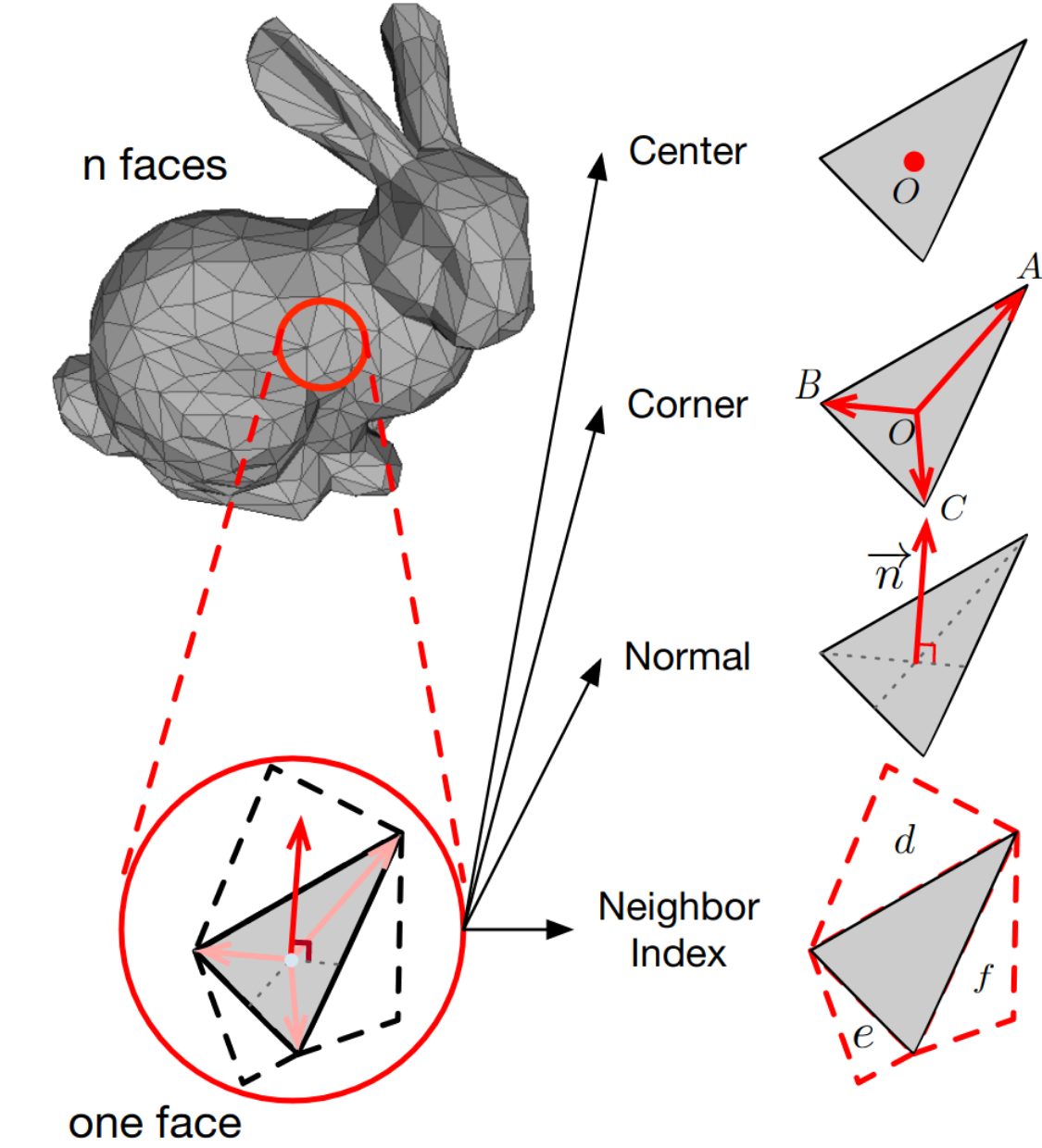
A convolution-like operation is then defined on the center-to-corner vectors, but instead of translation, one rotates clockwise through all pairs of vectors, multiplying them with a weight matrix and pooling the results. The center positions are processed using a shared MLP as in PointNet. The aggregated structural features are then combined with the spatial features to form the proposed Mesh Convolution.
Building up a deep architecture around this new operator, MeshNet outperforms Multi-View CNN and PointNet++, two of the strongest baselines at the time of publication. It is also almost as fast as PointNet and very robust to changes in mesh structure and density.
MeshCNN
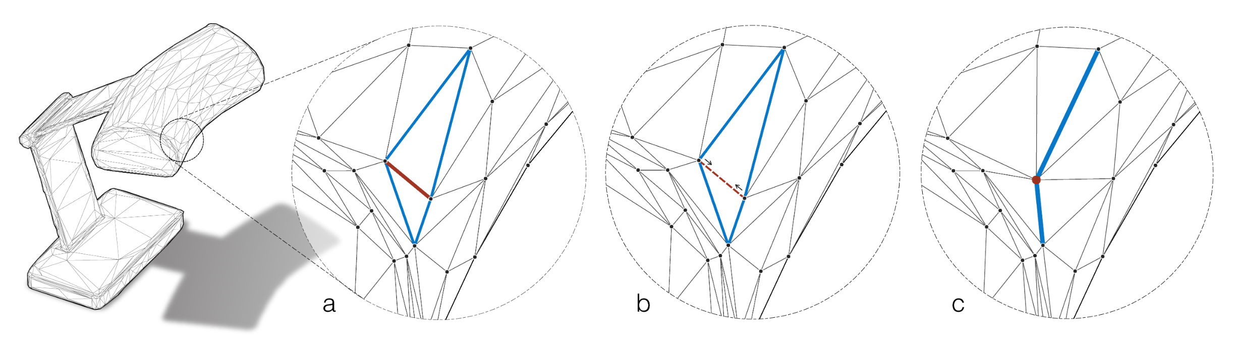
Similar to the previous architecture, this one is also specifically designed to handle the peculiarities of meshes, but the basic building blocks are now edges instead of faces. Each edge in a mesh takes part in two triangles on which both a novel convolution and pooling operation is defined.
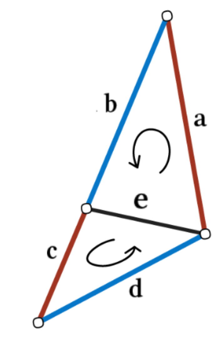
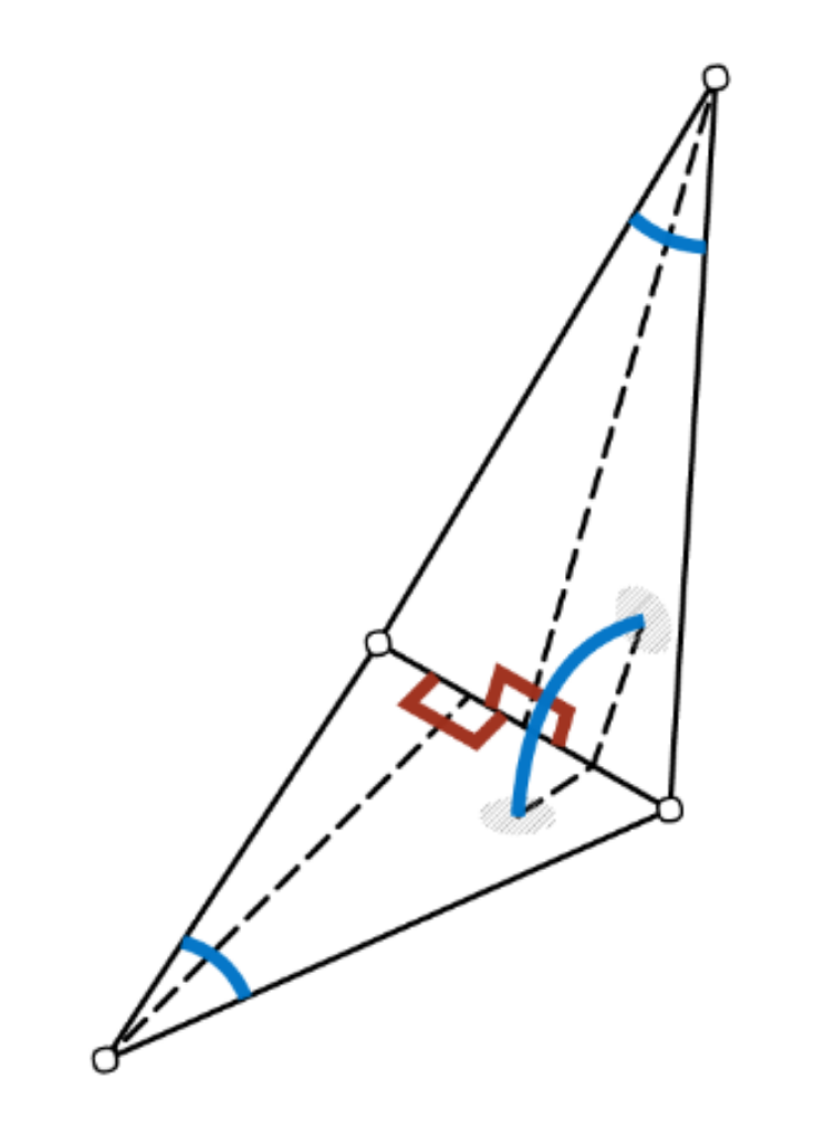
The convolution is defined similarly to MeshNet over the participating edges. To obtain order invariance, edge feature pairs are passed through a symmetric function like summation. Edge features are again hand-crafted and contain two inner angles, the angle between both triangles and two edge length ratios as depicted below, which need to be sorted to resolve order ambiguities. Those features are chosen specifically to be invariant to translation, rotation and scale as they are all relative, i.e. without referencing surrounding information.
Because both convolutions and pooling are implemented, MeshCNN behaves much like a “normal” CNN, building hierarchical features with increasing depth while increasing the receptive field. And because the pooling operation can be reversed, we can even build fully convolutional networks for semantic segmentation. Unfortunately, the authors didn’t evaluate their model on the de facto standard benchmark datasets ModelNet40 for classification, and ShapeNet for semantic segmentation, but a quick look online revealed, that both datasets are not manifold, meaning there could be edges with more than two adjacent triangles, which breaks the assumption made in designing MeshCNN.
DGCNN
The final work I want to discuss in this article could just as well have appeared in a previous post on point cloud learning, as this is what the Dynamic Graph CNN takes as input, but I decided to flout the conventions and discuss it hear, because in name and at heart its a real graph approach.
In contrast to other works, including those featured above, DGCNN creates its own dynamic graph on the fly during execution. To do so, for each input point, the nearest neighbors are found in each layer, which means that proximity is defined in feature space as opposed to Euclidean space for all but the very first layer. Instead of using the features attached to each point, like position, color or normals, new pair-wise edge features are computed.
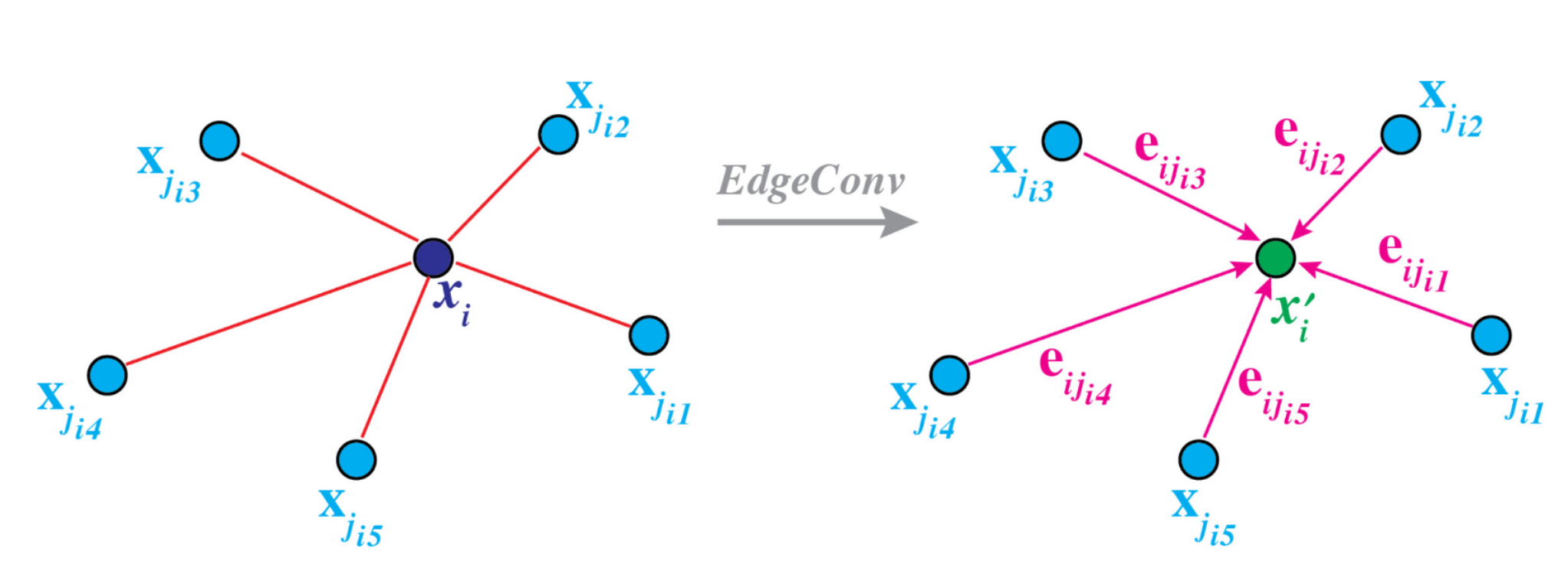
For the input, these are simply the difference between the position of each pair of points as well as the position of the center point. The former is multiplied by the networks weights, while the latter is multiplied by a bias and added to the product. Passing everything through a ReLU non-linearity we obtain our edge features. Adding those up yields the standard convolution operation—now dubbed EdgeConv—were the output is used as input features for the subsequent layer.
You might wonder why we need to use pairs of points to compute our features instead of directly using the features of individual points, which, as it turns out, is what PointNet and PointNet++ do. The downside of this approach is, that local neighborhood information is ignored as every point is processed individually. As we know from learning on images though, local information is crucial for building up more complex representations from simple primitives. Using both pairs of points and individual points, we can capture both local and global information at the same time.
Another difference to PointNet and PointNet++ is, that the neighborhood graph is computed in feature space as opposed to remaining in the original Euclidean space in which the farthest point sampling (or ball query) is performed. The implication is, that DGCNN (similar to image CNNs) can capture semantic similarity, i.e. small distance in feature space, instead of spatial similarity, allowing to detect reoccurring parts like wings or ears in deeper layers which can be comparatively far apart in the original space.
What’s next?
By now we have covered a lot of ground from point clouds over voxel grids to graphs. The final approach to learning from 3D data I want to cover is also the oldest and most obvious: Don’t bothering with three dimensions but instead projecting everything into 2D and applying our beloved and powerful standard CNN architectures. See you there.
Code: ![]()